Post-processing of Finite Element Results with FreeCAD and Paraview
Introduction
Some FreeCAD forum posts and tutorials use Paraview (PV) to review and analyse FreeCAD FEM Workbench results. This post explains the basics of transferring data from FEM Workbench to PV and shows some of the options and settings for displaying data.
Prerequisites
- FreeCAD version 0.19 or higher.
- Paraview downloaded directly from it's website or your preferred package manager.
- This post is based on Paraview version 5.8.0 for Windows, which was the most recent version at the time of writing the post.
- The FreeCAD files used for this post available in this and this FC forum thread.
Data Transfer from FEM workbench
In FEM workbench highlight the CCX_Results object. Next, use menu option File > Export > FEM result VTK (*.vtk *.vtu) to export the VTK data.
Data Import in Paraview
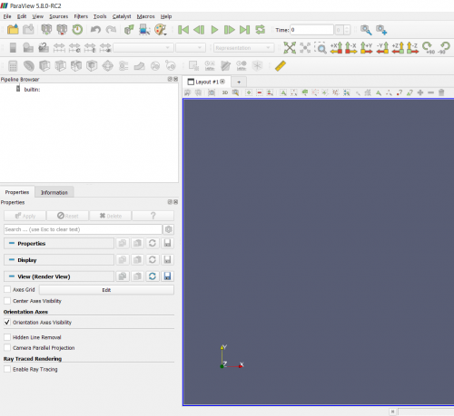
The start-up screen shows an empty Pipeline Browser. This is where the imported VTK data objects and applied filter objects (for geometry or data) will be visible.
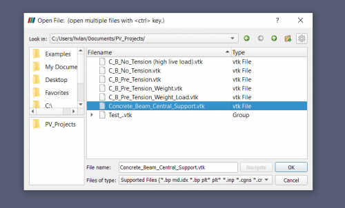
Use menu option File > Open > *.vtk to open the VTK file that was generated with FEM Workbench.
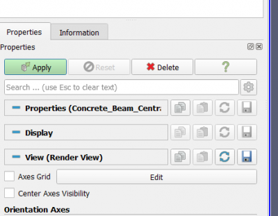
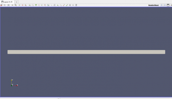
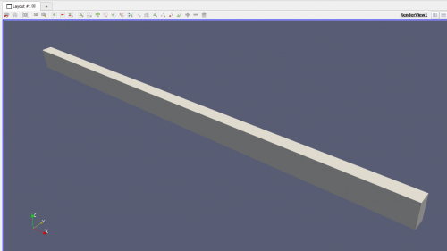
Press Apply on the properties tab. By default, this will show a top view (looking down along z-axis) of the geometry.
The gray geometry can be inspected by rotating the view. The left mouse button makes the geometry swivel, but unfortunately in a difficult-to-control way (compared to FreeCAD). To get a predictable rotation hold the X, Y or Z key while dragging the mouse with left mouse button pressed to rotate the model around the X, Y or Z axis, respectively
Saving/Loading State
Rather than saving data, Paraview stores the status (state) of the actions performed on the imported VTK object. Therefore, to save your work use menu option File > Save State. NOTE: there will be no warning when leaving Paraview to save the state and all work may be lost when exiting the program.
To continue where you left off in the previous session use File > Load State. This prompts the user to specify a VTK file, which means that the actions performed in the last session can also be applied to a new VTK file. In this way, data from different FEM Workbench analyses can be displayed in exactly the same way, without any additional effort.
Visualise FEM Workbench Results
Paraview has many options and settings for displaying results. We will first have a look at displaying base import data on the original geometry and thereafter see how to apply filters to modify the geometry. Finally, we will use the calculator and integration filters to derive new results by combining base import data.
Base Data Displayed on Original Geometry
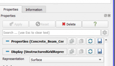
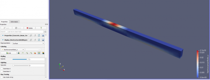
As the pipeline browser can contain several VTK objects and filter objects, first confirm that the right VTK object is highlighted in the pipeline browser. The selections and settings for displaying this VTK object can now be found on the Properties Tab. To make sure all settings are visible and aligned with this post press the Advanced Settings button (the gear wheel icon on the below picture).
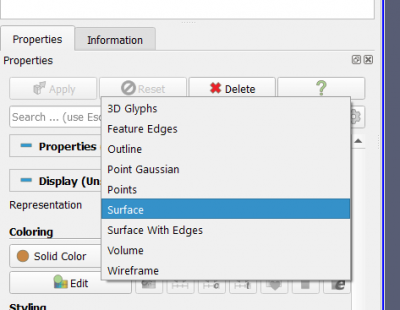
The first setting that we can change is the way data is presented on the geometry. This is done on the Representation drop down menu. For now we will only use the Surface or Wireframe option.
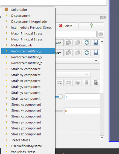
So far no results are displayed. For this we need to change the Coloring option. The default is Solid Color, but the drop down menu shows all the scalar data that is available in the imported VTK file.
For the purpose of this post we choose ReinforcementRatio_x, but it is easy to change to any data type.
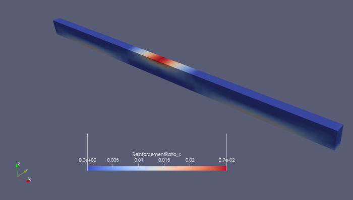
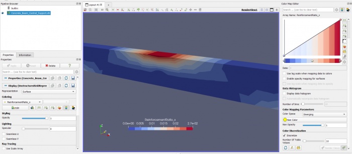
The RenderView window will now show an iso-plot of the selected data type and a Color Legend of the data range.
The Color Legend can be dragged around the screen to a more convenient location and will change orientation when nearing any of the windows edges.
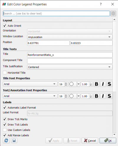
Alternatively, the settings of the color legend can be controlled in great detail by opening the Edit Color Legend Properties dialogue from the Properties Tab (press last Icon to the right)
This opens the following window for the color legend settings
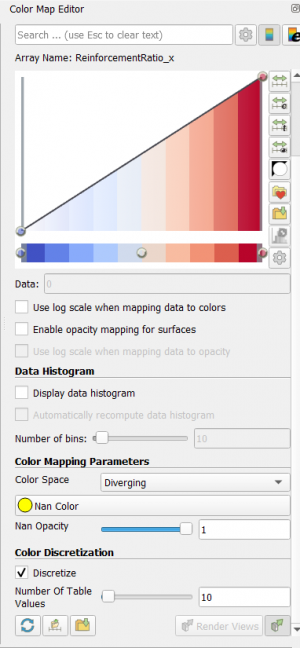
The coloring of the iso map can be controlled through the Color Map Editor, which is activated by pressing the Edit button on the Properties Tab:
The setting for Color Discretization is useful to limit the number of iso values, thus creating more practical ranges for design. The default number of ranges is 256, but here the number is set at 10.
Applying Filters to FEM Workbench results
To modify the base data or geometry imported from FEM Workbench, filters can be applied.
Here only the Slice and Warp filters will be discussed. Filters for creating compound results from base data will be discussed in the next section.
To apply the Slice filter, highlight the VTK object that needs to be sliced and press the Slice Icon. Alternatively, find the Slice filter in the menu Filters > Alphabetical. This adds the Slice filter object to the Pipeline Browser and the location in the tree shows that it is applied to the VTK object. The position in the tree matters, because filters can be applied to different VTK objects or even to other filter objects. The filter object cannot be dragged around in the tree to change the object it is applies to. The target object can only be changed through the menu (or by right-clicking) option Edit > Change Input.
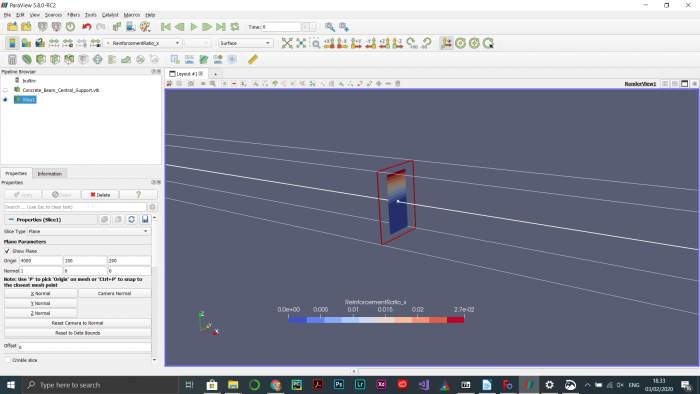
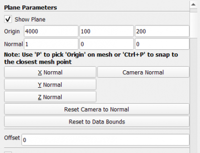
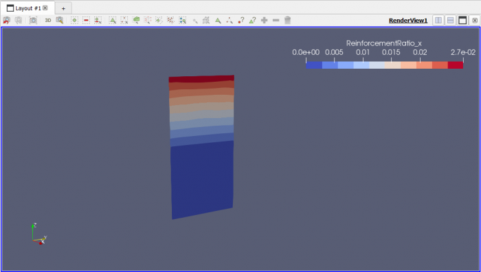
The location and orientation of the slice can be modified by dragging the slice and its normal vector with the mouse or through the Properties tab. In the below figure the origin of the slice has been placed at the center of the beam (over the central support) and the normal to the plane points in the x-direction.
To get rid of the bounding boxes deselect the Show Plane box at the top of the Plane Parameters dialogue.
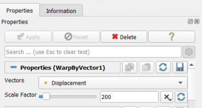
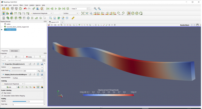
The Warp by Vector filter can be used to display the deformed geometry. Highlight the VTK object and press the Warp by Vector Icon. This adds the filter to the Pipeline Browser. Alternatively look for the filter in the menu Filters > Alphabetical. Next select Displacement in the Vectors drop-down menu of the Properties tab and set an appropriate scale factor. Don’t forget to press the Apply button after changing the settings.
The maximum displacement value is 0.98 mm.
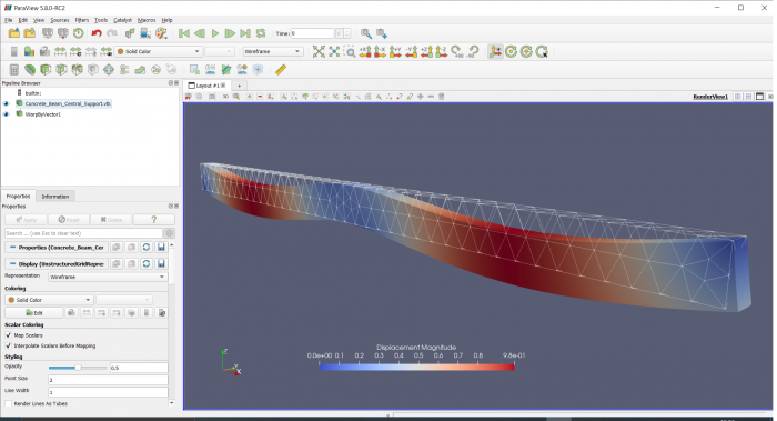
To show the deformed geometry superimposed on the undeformed geometry, simply make both the VTK object and Warp filter object visible by clicking the eye icon next to it. In the following picture the Representation setting for the VTK object was changed to Wireframe and the Opacity reduced to 0.5 to prevent it from obscuring the Deformed geometry.
NOTE: As more objects are added to the Pipeline Browser and more display windows are open, it becomes increasingly important to ensure that the right object is selected in the Pipeline Browser and the right Window has focus when making changes to the Properties Tab. Otherwise much time can be spent on finding the right property or changes to properties may not seem to take effect.
Applying Filters to Derive Compound Results from Base Import Data
If we want to know the amount of reinforcement steel in the beam as a whole or the amount passing though a particular cross section we need to perform integration (summation over the geometry) of the base data.
For example, the total volume of reinforcement bars in the beam running in x-direction is obtained from the integral INTEGRATE(ReinforcementRatio_x * dx * dy * dz)
over the full geometry and the total area of reinforcement steel
running though a particular beam cross section is obtained from INTEGRATE(ReinforcementRatio_x * dy * dz) over a slice.
In Paraview, integration can be done with an Integration Filter. This filter can be applied to the entire VTK object (the beam) or to a Slice (the cross section).
NOTE: due to a mismatch of node ordering between FCFEM and PV, integration over a volume renders negative results, i.e. INTEGRATE( 1.0 * dx * dy *dz) = - Volume instead of + Volume.
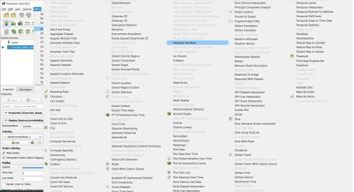
To calculate integrals we need to apply an Integration Filter, which can be found in the menu item Filters > Alphabetical. Highlight the VTK object and apply the filter.
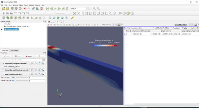
Press the Apply button in the Properties tab and the results will open in a separate window to the right of the Renderview.
Before we tidy this up to find the desired result, i.e. INTEGRATE(ReinforcementRatio_x * dx * dy * dz), lets first see how we can control where the window is placed and what it contains.
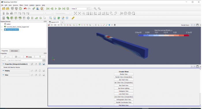
First close the SpreadSheetView window that has opened to the right. Then press the horizontal split icon on the Renderview window and a new window will open with a menu of display options. Before selecting an option, make sure the Integration filter object is highlighted in the Pipeline Browser.
To display numerical results we need to select SpreadSheet View at the bottom of the Create View list. This generates a spreadsheet of all available results in the VTK object integrated over the volume.
To inspect INTEGRATE(ReinforcementRatio_x * dx * dy * dz)
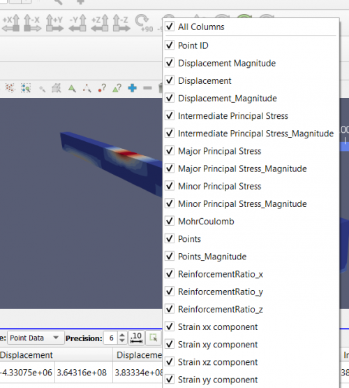
we could scroll to the right through the table, but we can also remove
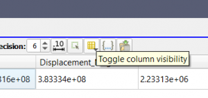
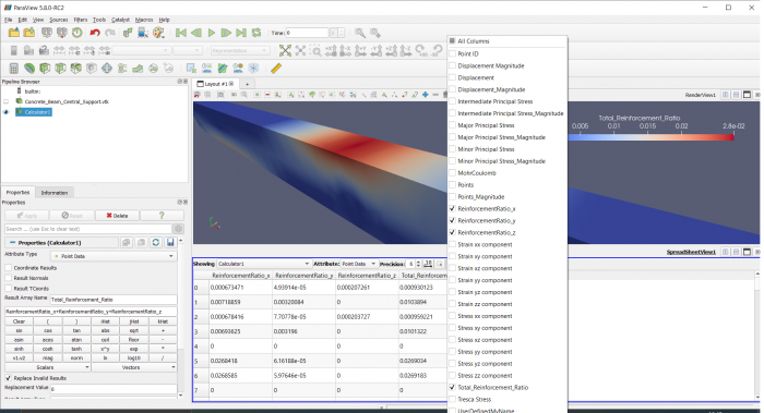
all unwanted results by deselecting them, i.e. deselect All Columns and
select ReinforcementRatio_x.
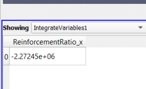
Now we are left with just one value in the table of integration results
As explained before this is the negative value of the integral we are looking for. So the indicative total volume of steel required in x direction is 2.27e+06 mm3 (= 2272 cm3) or 2272 cm3 * 7.6 g/cm3 = 17267 g (= 17.3 kg). In practice the number will be higher due to practical considerations (e.g. anchoring requirements, minimum reinforcement requirements, etc.). Nevertheless, this result can be used to compare conceptual designs
The above was an example of the integration of a variable directly exported by FEM Workbench. In some cases we may want to combine VTK variables to obtain new results. This can be done in several ways, but here I will only discuss the simplest, i.e. with the Calculator Filter.
For example, if we want to know the total reinforcement requirement in all three coordinate directions we would have to sum ReinforcementRatio_x, ReinforcementRatio_y and ReinforcementRatio_z.
The Calculator filter can be found as an icon on the left of the filter bar or via the menu Filters > Alphabetical. The name for the resulting variable can be entered in field Result Array Name. Here we name the result Total_Reinforcement_Ratio. The formula can be composed in the box below the Result Array Name field. Input values can be selected from the Scalars drop down menu and they can be combined into a formula for the result using the operators given. After pressing the Apply button, the result will be available as a new variable in any subsequent operations (e.g. an Integration Filter) or views (e.g. RenderView or SpreadSheetView, see below).
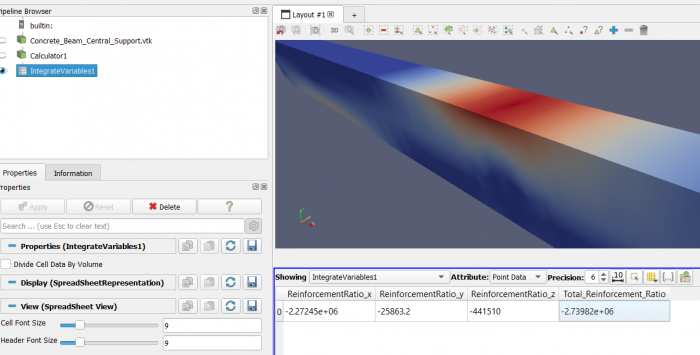
For example, we can now apply the integration filter to the new variable Total Reinforcement Ratio
This shows how the total reinforcement requirement compares to those in the individual coordinate directions.
Integration over a Slice
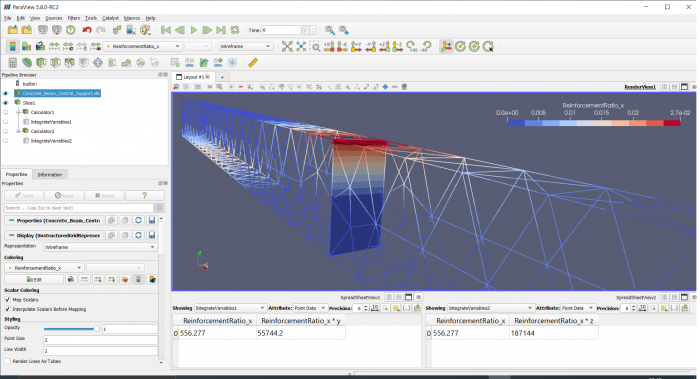
In the previous section we discussed the Integration filter and its application to the entire VTK object. To demonstrate integration over a slice we will in this section determine the total reinforcement requirement and its center of gravity for the central cross section of the beam. The end result is shown in the picture below. The interaction of various objects can be inspected in the Pipeline Browser. The slice filter is applied to the beam VTK object and two Calculator filters are applied to the slice filter to derive the new variables “Reinforcement_ratio_x * z” and “Reinforcement_ratio_x * y” from the base data. These variables need to be integrated to determine the center of gravity of the reinforcement. Finally, Integration filters are applied to each Calculator to integrate results over the Slice. Please refer to the previous section for a general introduction of the Integration filter and its settings.
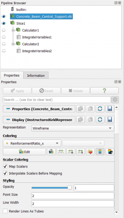
Apply the following Settings in the Properties tab for the VTK object:
| Properties Tab Settings | Comment |
|---|---|
| Representation: Wireframe | So the Slice is visible |
| Coloring: ReinforcementRatio_x | Or any other color |
| Styling > Line Width: 2 | Or any other setting that gives a pleasing result |
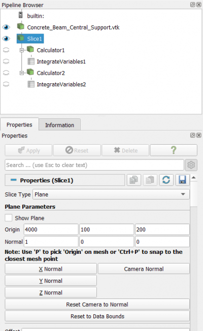
Next highlight the VTK object and apply a Slice filter with the following settings on the Properties tab
| Properties Tab Settings | Comment |
|---|---|
| Plane Parameters > Show Plane: deselect | Remove the bounding boxes |
| Plane Parameters > Origin: 4000 / 100 / 200 | Position of central section |
| Plane Parameters > Normal: 1 /0 /0 | Normal of Slice points in x -direction |
| Coloring: ReinforcementRatio_x | Optional |
| Styling > Line Width: 2 | Or any other setting that gives a pleasing result |
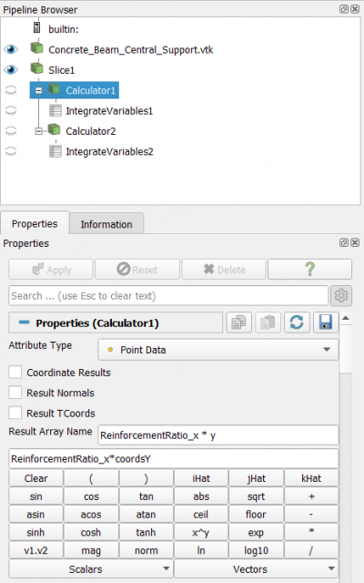
Settings Calculator 1
Calculator 1 computes the new variable ReinforcementRatio_x * y which needs to be integrated to obtain the y-coordinate of the reinforcement’s center of gravity.
After pressing Apply, a new variable named “ReinforcementRatio_x * y” is available for display or further processing.
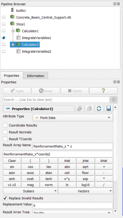
Settings Calculator 2
Calculator 2 computes the new variable ReinforcementRatio_x * z which needs to be integrated to obtain the z-coordinate of the reinforcement’s center of gravity.
After pressing Apply, a new variable named “ReinforcementRatio_x * z” is available for display or further processing.
Finally, two Integration filters are applied, one on Calculator1 to integrate variable ReinforcementRatio_x * y and on Calculator2 to integrate ReinforcementRatio_x * z. Each are displayed in their own window with SpreadSheetView selected. The way to deselect all other results is explained earlier.
Finally the Center of Gravity can be calculated from the above results as:
CoG_y = 55744.2 / 556.277 = 100.2 mm (exact value: 100 mm)
CoG_z = 187144 / 556.277 = 336.4 mm (exact value: 5/6 * 400 mm)
Integration over a Line
To demonstrate visualisation and integration of results over a line we use the 2D example of a heavy wall as introduced in this FC forum thread. The FreeCAD file for this example can be downloaded in this FC forum thread. The challenge is to visualise reinforcement ratio across various vertical cross sections and to determine the required area of steel from integration of those results.
Techniques introduced in previous sections of this post will not be repeated here. It is also important to note again that as more objects are added to the Pipeline Browser and more display windows are open, it becomes increasingly important to ensure that the right object is selected in the Pipeline Browser and the right Window has focus when making changes to the Properties Tab. Otherwise much time can be spent on finding the right property or changes to properties may not seem to take effect.
Starting with the VTK object imported from FEM Workbench, we note that the PV controls operate slightly differently on a 2 dimensional object. The left mouse button drags the geometry and the middle mouse button rotates it. To position the geometry in the plane of analysis (i.e. x-y), press the icon that puts the view along the negative z axis:
For the picture below the Coloring property on the Properties tab for the VTK object was set to ReinforcementRatio_x.
The only additional object required to visualise a variable along a straight line is a Plot Over Line filter. This can be activated from the icon bar or the menu option Filters > Alphabetical.
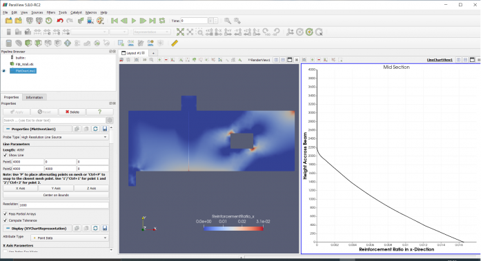
We next want to display the horizontal reinforcement requirements in the vertical cross section under the column. To achieve this in the way shown below, the following settings need to be changed in the Properties tab of the Plot Over Line filter (make sure the LineChartView window and the Plot Over Line object both have the focus)
| Properties Tab Settings | Comment |
|---|---|
| Line Parameters > Point 1: 4000 / 0 / 0 | Point at bottom of wall under the column |
| Line Parameters > Point 2: 4000 / 4000 / 0 | Point at top of wall under the column |
| x Axis Parameters > x Array Name: ReinforcementRatio_x | Displays ReinforcementRatio_x on the horizontal axis |
| Series Parameters: tick “arc length” only | This is the length parameter along the line |
| Title > Chart Title: Mid Section |
|
| Annotation > Show Legend: deselect | Meaningless for the current choice of vertical axis |
| Left Axis > Left Axis Title: Height Across Beam |
|
| Left Axis Range > Use Custom Range: deselect | Deselect to maximise the data range along the axis |
| Bottom Axis > Bottom Axis Title: Reinforcement Ratio in x-Direction |
|
| Bottom Axis Range > Use Custom Range: deselect | Deselect to maximise the data range along the axis |
Note that the distance along the line (arc length) is usually on the
horizontal axis and the variable that we want to display (here
ReinforcementRatio_x) on the vertical axis. However, as the wall section
in this example is vertical and we want to see the reinforcement
requirement over the height of the wall, it is more natural to inverse
the axes. This, however, comes at the expense of a lot more changes to
the settings in the Properties tab for the Plot Over Line filter.
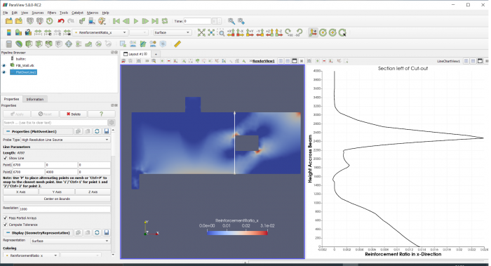
In the next two picture only the location of the line was changed. Note
however that this relocation will automatically change the Left Axis
Range > Use Custom Range setting to “select”. This may mean that the
graph does not properly fit in the LineChartView window. It is therefore
necessary to deselect this option every time the position of the line
is changed. Other settings are as per the above table.
| Properties Tab Settings | Comment |
|---|---|
| Line Parameters > Point 1: 6700 / 0 / 0 | Point at bottom of wall under left side of cut-out |
| Line Parameters > Point 2: 6700 / 4000 / 0 | Point at top of wall above left side of cut-out |
| Title > Chart Title: Section left of Cut-out |
|
| Left Axis Range > Use Custom Range: deselect | Deselect to maximise the data range along the axis |
| Bottom Axis Range > Use Custom Range: deselect | Deselect to maximise the data range along the axis |
| Properties Tab Settings | Comment |
|---|---|
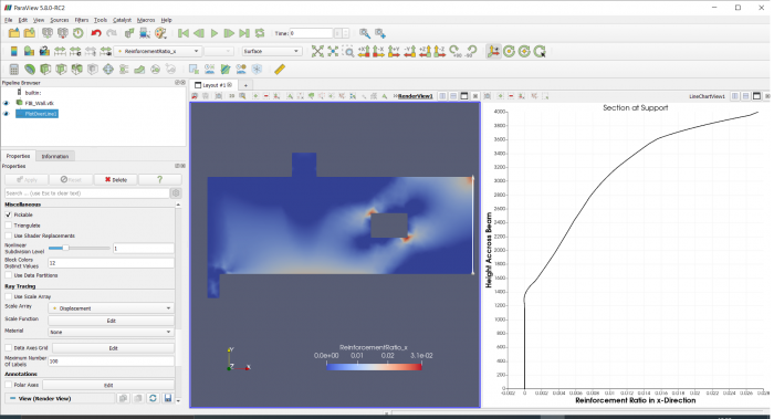
| Line Parameters > Point 1: 10950 / 0 / 0 | Point at bottom of wall at right-hand support |
| Line Parameters > Point 2: 10950 / 4000 / 0 | Point at top of wall at right-hand support |
| Title > Chart Title: Section at Support |
|
| Left Axis Range > Use Custom Range: deselect | Deselect to maximise the data range along the axis |
| Bottom Axis Range > Use Custom Range: deselect | Deselect to maximise the data range along the axis |
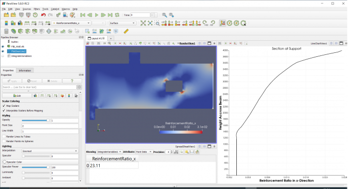
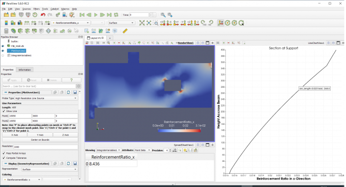
The total horizontal reinforcement requirement in the last cross section can now simply be obtained by applying an Integration filter to the Plot Over Line object, i.e. highlight the Plot Over Line object in the Pipeline Browser and add an Integration filter from the menu option Filters > Alphabetical.
In the usual way deselect all but the ReinforcementRatio_x result in the SpreadSheetView and read off the result as 23.11 mm2 / mm. To obtain the total cross sectional area of steel, we still need to multiply with the thickness of the wall, which in this example is (an impressive) 600 mm. So the total cross sectional area of steel running through the cross section near the right hand support is 23.11 * 600 = 13866 mm2 = 139 cm2
To achieve a more practical distribution of reinforcement we could integrate the above graph in parts. For example, if we want to know the required cross sectional area of steel in the top 400mm of the wall then we should adjust the properties of the Plot Over Line object as follows
| Properties Tab Settings | Comment |
|---|---|
| Line Parameters > Point 1: 10950 / 3600 / 0 | Point near top of wall at right-hand support |
| Line Parameters > Point 2: 10950 / 4000 / 0 | Point at top of wall at right-hand support |
| Left Axis Range > Use Custom Range: deselect | Deselect to maximise the data range along the axis |
| Bottom Axis Range > Use Custom Range: deselect | Deselect to maximise the data range along the axis |
This yields the following result
The result for the top 400 mm of the wall is thus 8.436 mm2 / mm. So the top 10% of the wall requires 8.44 / 23.11 * 100% = 37% of the reinforcement steel.
This procedure could be repeated to divide the wall in zones of constant reinforcement.
Representation of Vector Results with the Glyph 3D Filter
So far we have only dealt with Scalar values, like reinforcement ratio and displacement magnitude. Visualization of vector results, like Principal Stress vectors, is done with Glyphs.
Let’s return to the VTK data object for the beam with central support and visualize maximum and minimum principal stress vectors.
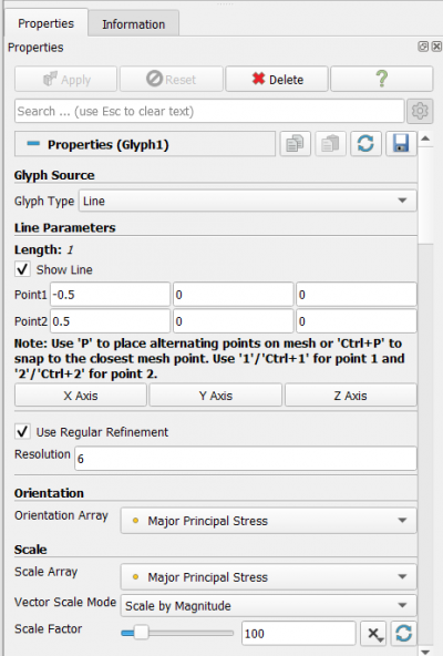
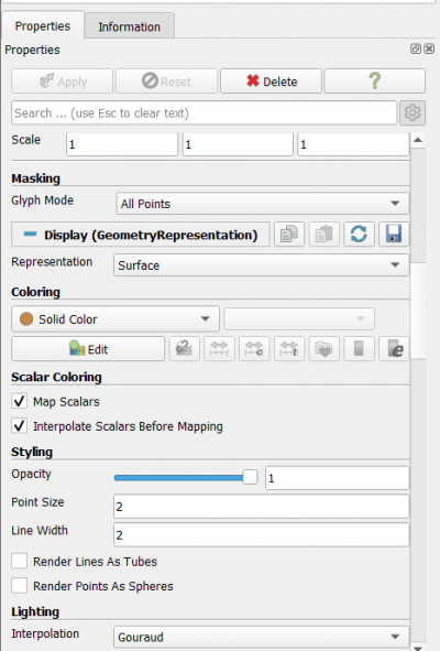
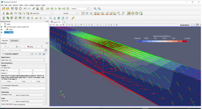
Highlight the VTK data object in the Pipeline Browser and select the Glyph Filter from the Filter Icon bar or from the menu option Filter > Alphabetical. Then apply the following settings in the Properties tab of the Glyph Filter object (see table and picture):
| Properties Tab Settings | Comment |
|---|---|
| Glyph Source > Glyph Type: Line | Unfortunately there is no option for a double sided arrow |
| Orientation > Orientation: Major Principal Stress | The Glyph takes the principal stress direction |
| Scale > Scale Array: Major Principal Stress | The length of the line will represent the magnitude of the principal stress |
| Scale > Vector Scale Mode: Scale by Magnitude |
|
| Scale > Scale Factor: 100 | Or any other setting that gives a pleasing result |
| Masking > Glyph Mode: All Points | To make sure the stress in every node is displayed |
| Coloring > Solid Color | A single color gives greatest clarity of “stress flow” |
| Coloring > Edit > Green | Or any other setting that gives a pleasing result |
| Styling > Line Width > 2 | Or any other setting that gives a pleasing result |
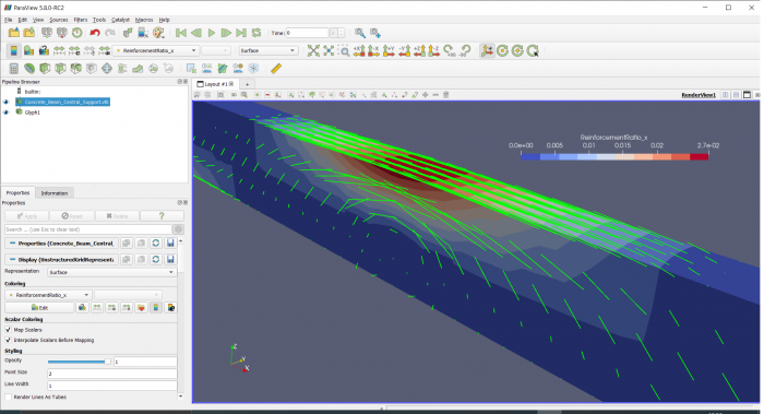
If all goes well you should see the following result for the example file.
Next add another Glyph Filter with the following settings for the Minor Principal Stress (don’t forget to first highlight the VTK data object in the Pipeline Browser):
| Properties Tab Settings | Comment |
|---|---|
| Glyph Source > Glyph Type: Line | Unfortunately there is no option for a double sided arrow |
| Orientation > Orientation: Minor Principal Stress | The Glyph takes the principal stress direction |
| Scale > Scale Array: Minor Principal Stress | The length of the line will represent the magnitude of the principal stress |
| Scale > Vector Scale Mode: Scale by Magnitude |
|
| Scale > Scale Factor: 100 | Or any other setting that gives a pleasing result |
| Masking > Glyph Mode: All Points | To make sure the stress in every node is displayed |
| Coloring > Solid Color | A single color gives greatest clarity of “stress flow” |
| Coloring > Edit > Red | Or any other setting that gives a pleasing result |
| Styling > Line Width > 2 | Or any other setting that gives a pleasing result |
The final result shows the major and minor principal stress vectors superimposed on the beam with ReinforcementRatio_x.
Export of Graphical Results
To export a RenderView window highlight the window and use menu option File > Save Screenshot






Comments
Post a Comment